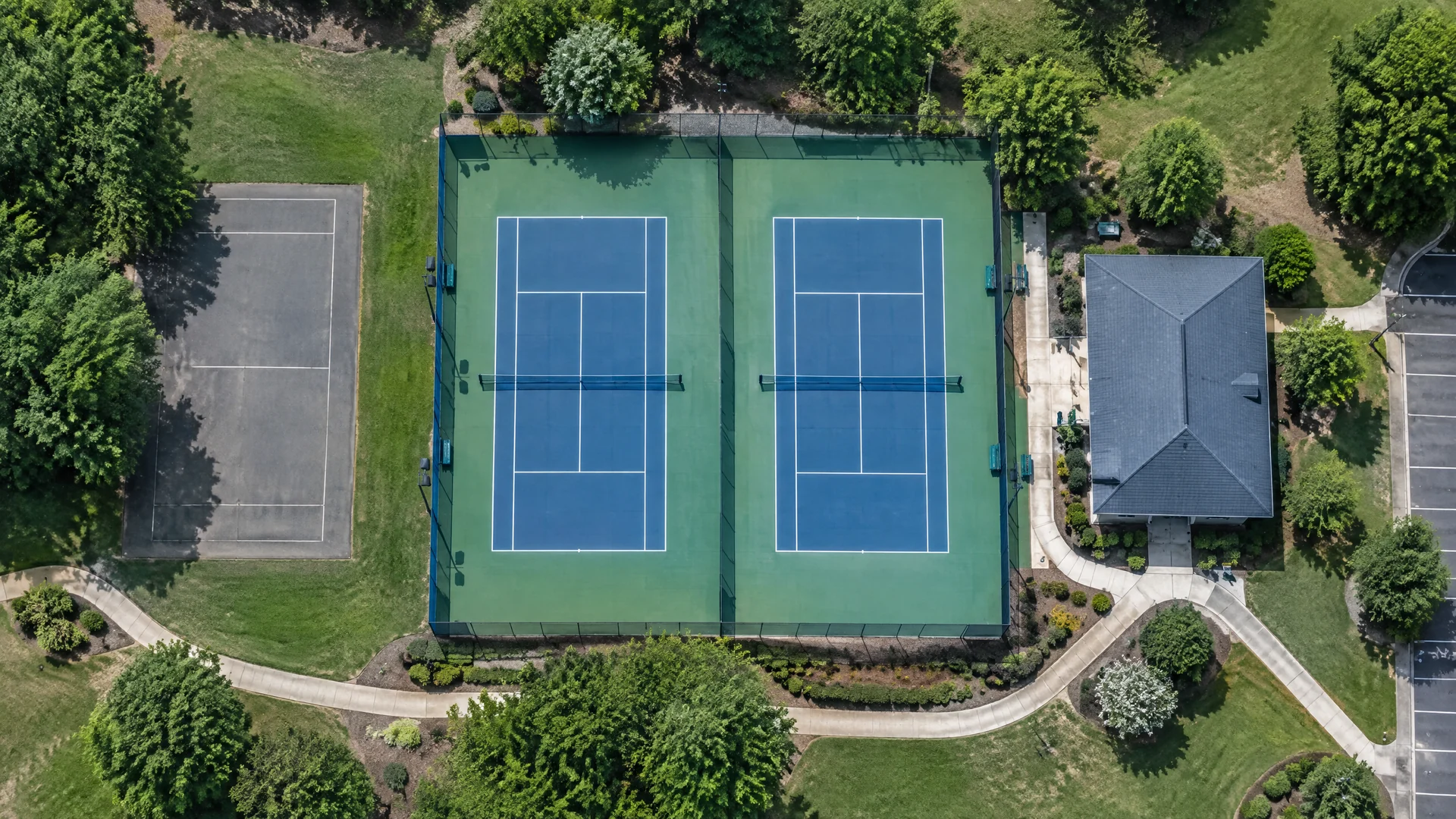
Tennis court detection uses computer vision to turn a dated overhead image into candidate locations for review. Rather than “seeing” a court like a person, a model learns features from labelled pixels and estimates whether a patch, box or polygon is court-like. Its dependable output is a review queue and, after checking, a map—not a claim that every court in an area has been found.
This guide explains the technical decisions behind tennis court detection in aerial imagery: what the imagery can resolve, how labels and coordinates change the task, why evaluation can be misleading, and where a person must remain in the loop. It is about remote sensing sports facilities, not match analysis. For the wider decision context, see the Sports Technology Guide.
Tennis court detection is not on-court player tracking
Remote sensing observes facilities from above, typically using imagery collected by aircraft, drones or satellites and then referenced to the ground. The unit of interest is a relatively fixed physical asset: a court, its footprint, its surface and nearby features. A tennis court may be visible as a rectangle with line markings, fencing, lighting, surrounding run-off area and neighbouring courts. The task can support an inventory or a planning map even when no people are present.
That is different from an on-court system that detects players, ball trajectories or line positions during play. Those systems use a different viewing geometry, timing requirement and definition of success. A still orthophoto might establish that a facility existed when the image was taken; it cannot establish current occupancy, match activity, coaching quality or player movement. For that distinction, read Computer Vision in Sports: What Cameras Can Really Tell Coaches and How AI Video Analysis Works in Sports.
This scope matters before any model is chosen. If the question is “Where are potential courts in a municipality?” a georeferenced aerial-image workflow is appropriate. If the question is “Which court is free right now?” it is not. The first needs imagery provenance, spatial labels and human map review; the second would require current operational data that an aerial detection model does not provide.
Start with the image: platform, age and ground sample distance
“Aerial” and “satellite” are not interchangeable descriptions of usable detail. An aerial orthophoto is an image corrected so it can carry map-like geometry; a raw aerial photograph may still have displacement from terrain or camera tilt. Satellite imagery can be valuable for broad land-cover monitoring, but its pixel size may be too coarse to make a tennis court a reliably separable object. The right choice depends on the imagery’s ground sample distance (GSD), bands, date, look angle, processing and licence—not only on the platform name.
GSD is the ground distance represented by one pixel, not a promise that an object at that scale can be identified. A full-sized tennis court is 23.77 m long under the ITF Rules of Tennis. At 0.5 m per pixel, that length spans about 47.5 pixels in a perfectly oriented image (23.77 ÷ 0.5). This scale illustration is not a performance threshold: shadows, compression, oblique viewing, vegetation, paint contrast and court condition can still obscure the pattern.
By contrast, the visible bands of Sentinel-2 are sampled at 10 m, so a 23.77 m court length would span roughly 2.4 pixels before considering orientation or context. That does not make satellite data useless; it makes it poorly matched to a generic court-footprint detector at that resolution. Fine aerial imagery may offer more useful detail, but varies by season, sensor and jurisdiction. Always record the acquisition date, nominal GSD, coordinate reference system, provider and processing level before comparing sources.
| Characteristic | Why it changes the result | Practical review question |
|---|---|---|
| Acquisition date | Courts can be resurfaced, covered, demolished or newly built | Does the image date fit the planning question? |
| GSD / pixel size | Controls how much court geometry is sampled | How many pixels span the expected court length and width? |
| Orthorectification and coordinates | Enables sensible map placement and distance checks | Is the image an orthoimage with usable spatial reference? |
| Bands, season and illumination | Affect surface colour, line visibility, shadows and vegetation | Do training and target images differ materially? |
| Licence and permitted use | Governs storage, model training, derivative maps and publication | Does the licence cover each proposed use and sharing route? |
Choose classification, detection or segmentation deliberately
The word “detect” hides three different machine-learning tasks. Classification assigns one label to a whole image chip: for example, “contains a tennis court” or “does not contain a tennis court.” Object detection predicts one or more boxes and a class, which is useful when the aim is to propose individual courts. Instance segmentation draws a separate pixel mask for each court, which can support a more precise footprint when labels and imagery justify that precision.
A scene-classification dataset can be useful for learning broad visual cues, but it is not automatically a court inventory dataset. The UC Merced Land Use Dataset, for example, is a 21-class research dataset that includes a tennis-court class. Its images were manually extracted from USGS urban imagery, and the primary dataset page describes 256 × 256-pixel images with one-foot pixel resolution. It provides an instructive starting point for a classification problem, but the class label on a chip is not the same thing as a verified polygon or a count of every court in the chip.
Choose the simplest output that answers the operational question. A facilities team prioritising sites for inspection may only need candidate boxes and confidence rankings. A mapping project that must estimate surface area may need reviewed segmentation polygons. More detailed labels increase annotation effort and create more ways to be wrong, particularly where fences, shared run-off areas or closely packed courts blur boundaries. This mirrors a general lesson in sports technology decisions: specify the decision first, then select the system output.
| Task | Label supplied during training | Typical output | Appropriate use | Important limitation |
|---|---|---|---|---|
| Classification | One class per image chip | Court-likely / not-court-likely score | Screening tiles | Does not locate or count individual courts reliably |
| Object detection | One box per court instance | Boxes, classes and confidence scores | Candidate inventory and review queue | Boxes can overlap, duplicate or include surrounding space |
| Instance segmentation | One mask per court instance | Pixel-level court outlines | Reviewed footprint or surface analysis | Boundary quality depends heavily on label rules and image detail |
Teach the model court geometry and local context
Useful labels show both the positive object and the cases that resemble it. A hard court may appear as a coloured rectangle with bright linework, but colour alone is fragile. Roofs, parking bays, multi-use games areas, swimming-pool surrounds and rectangular paved yards can all create similar shapes. Line markings, twin-court layouts, fencing, nets, access paths and the relationship to club buildings can add context, yet those cues also differ among regions and surface types.
Write an annotation guide before labelling. It should state whether the label represents the painted playing rectangle, the full fenced enclosure, a multi-court compound or an individual court. It should specify how to label grass, clay, hard, covered and disused facilities; how to handle partial occlusion; and when an unclear site is excluded rather than guessed. A reviewer should be able to apply the same rule to a tile without knowing which split it belongs to.
The associated geospatial record is as important as the picture. Preserve source ID, tile bounds, acquisition date, GSD, coordinate reference system, provider, licence, label version and reviewer decision alongside each annotation. Geospatial metadata documents the who, what, when, where, how and why of a data resource. That record lets a team trace a candidate back to its dated image rather than treating a cropped JPEG as self-explanatory.
Build a dataset that can test transfer, not memorisation
A model can appear accurate while recognising a familiar neighbourhood instead of a court. Randomly mixing nearby crops into training and test sets is a common route to this problem. Tiles from the same facility—or overlapping crops from the same original image—share lighting, surface colour, roofs, trees and local layout. If one crop is in training and its neighbour is in testing, the test score can be more flattering than performance in a new town.
Use a location holdout instead. Group images by facility, site, mosaic or geographic block before assigning train, validation and test sets, then reserve whole groups for evaluation. The test set should contain places the model has not seen and, when transfer is the goal, imagery conditions that matter in deployment. If labels come from several imagery providers or dates, record those groups too. A separate later-date holdout can expose errors caused by resurfacing, faded markings or changed surroundings.
The held-out set must also contain meaningful negatives. Include look-alikes such as basketball courts, solar-panel arrays, blue roofs and rectilinear paved areas, as well as ordinary non-court land. Include small facilities, dense urban sites, rural clubs and different surface colours where these are in scope. Dataset balance should reflect the decision: a broad-area search with few courts needs many credible negatives, otherwise a model can look good in a curated set but generate too many false alarms in the real search area.
Interpret confidence separately from measured accuracy
A confidence score is a model’s ranking signal for a particular prediction; it is not a measured percentage of correct courts in a city. Raising a threshold may reduce false positives, but it can also hide more true courts. A model that assigns “0.90” to a box is not automatically correct 90% of the time unless calibration has been demonstrated on comparable held-out data. Thresholds should therefore be selected against a documented review workload and error trade-off.
Precision and recall make that trade-off visible. Precision asks: among all candidate detections called positive, how many were confirmed? Recall asks: among all real courts in the review reference, how many were found? Accuracy alone is often misleading when courts are rare: a system that declares nearly every tile “not a court” can look accurate while missing the assets the project exists to find.
Here is a deliberately constructed manual-review example, not a reported model result. An independent reviewer establishes a reference of 24 unique courts in 40 held-out image tiles. After spatial matching and duplicate removal, the model produces 25 unique candidate detections: 18 match a reference court, seven are false positives, and six reference courts have no matching detection. Precision is 18 ÷ (18 + 7) = 72%; recall is 18 ÷ (18 + 6) = 75%. The precision denominator is all predicted positives, while the recall denominator is all actual reference courts.
| Review outcome | Count | Role in metric |
|---|---|---|
| Confirmed candidate matched to a reference court (true positive) | 18 | Numerator for precision and recall |
| Candidate that is not a court (false positive) | 7 | Added to the precision denominator |
| Reference court with no matched candidate (false negative) | 6 | Added to the recall denominator |
| Unique candidate detections | 25 | 18 + 7, the precision denominator |
| Independent reference courts | 24 | 18 + 6, the recall denominator |
Count courts only after spatial matching and human review
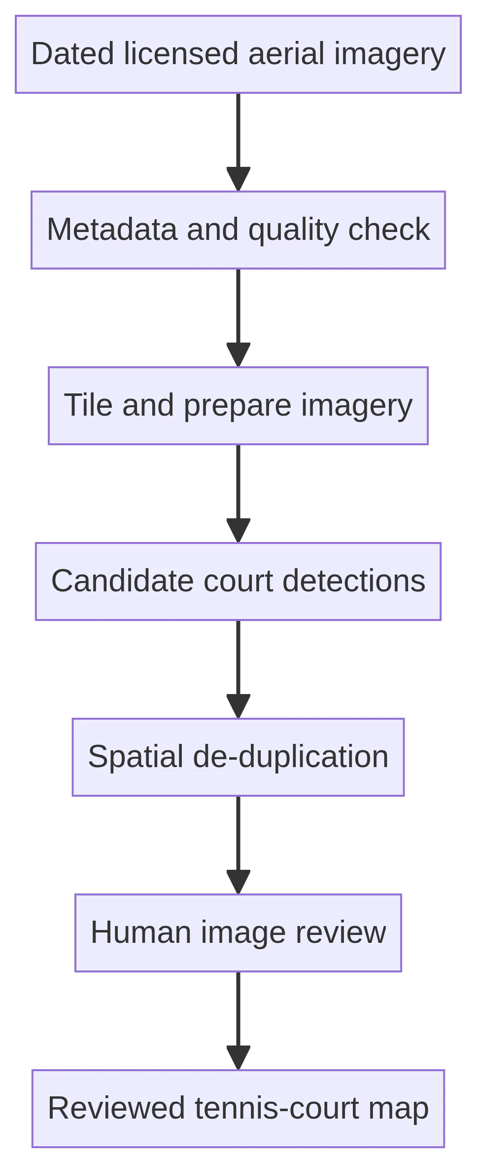
Tile boundaries and overlapping inference windows can make a single court appear more than once. Closely adjacent courts can also yield one oversized box or several partial boxes. A workflow needs spatial de-duplication before it reports a count: convert candidates to a common coordinate system, compare overlap or distance, retain the strongest candidate under a stated rule, and preserve the merge history. The result is a candidate count, not a verified facility count, until review is complete.
Human review should inspect the image at the relevant scale and log a decision such as confirmed, rejected, uncertain, merged duplicate or needs newer imagery. A reviewer may use authorised supporting records where the project permits, but must not silently convert uncertain evidence into a positive. Quality assurance benefits from a second reviewer on a sample of confirmations and rejections, especially around covered courts, faded surfaces and multi-sport facilities. This is the same discipline behind useful sports-science and training technology: an automated signal becomes useful only when a person can interpret its context and limits.
The final map should keep status fields rather than flattening every candidate into the same point. Separate “model candidate,” “human confirmed from imagery,” “uncertain,” “historical image only” and “rejected” records. Include review date, imagery date and reviewer rationale. That supports an auditable inventory, makes later correction possible, and prevents a map reader from mistaking a dated visual inference for a live service-status feed.
Use the output for planning, not live occupancy claims
A reviewed aerial inventory can help a council, club network or researcher identify areas for facility audits, compare broad distribution of courts, prioritise access checks, or create a fieldwork sampling frame. It can identify likely gaps that merit local verification. In a facilities programme, it may also help distinguish a single mapped complex from a dispersed set of sites before teams plan inspections or maintenance conversations.
It cannot show whether a court is open today, bookable, safe, publicly accessible, in use, privately restricted, maintained or compliant with competition rules. Image age is central here. USGS guidance, for example, notes that acquisition month and year are metadata for its orthoimagery products, and imagery programmes can be refreshed on multi-year cycles. A court’s surface, covering, fencing, markings or existence can change between capture and analysis.
Treat detection as one evidence layer among local records, site visits and responsible stakeholder input. That keeps the project focused on a defensible question—what may have been visible in a particular image at a particular time—rather than overstating it as a live locator. It also prevents confusion with video-based analysis, which is covered in AI video analysis in sports and serves a different operational purpose.
Respect licences, privacy and the limits of visual inference
Do not assume that an aerial or satellite image is free to train on, store, redistribute or display just because it is viewable online. Check the provider’s terms for model training, derivative datasets, map publication, attribution, sharing, retention and geographic restrictions. Some USGS-produced data are in the U.S. public domain, but USGS itself notes that not every image displayed on its sites carries that status. Commercial imagery and embedded third-party content need their own permission and licence review.
Privacy and proportionality also matter. A facility map can reveal information about small private sites or places connected to vulnerable groups. Collect only the fields needed for the stated planning purpose, avoid publishing imagery crops when there is no clear need, set access roles for source imagery and review records, and document retention. An imagery-derived point should never be used as the sole basis for a high-consequence decision about access, funding or a person.
The technical limitation is simple: a model can generalise only to the visual and geographic conditions represented—and responsibly labelled—in its data. It may fail on new surfaces, indoor facilities, partial covers, shadows, dense trees, snow, poor mosaics, uncommon court layouts or a different country. Re-test after changing provider, GSD, season, geography or label policy. A conservative, documented human-review step is not a temporary inconvenience; it is what turns tennis court detection aerial imagery into a useful and accountable mapping process.
A practical standard for a trustworthy court map
A trustworthy project begins with a precise question, dated licensed imagery and a label guide that says what counts as a court. It evaluates on held-out locations rather than neighbouring crops, reports precision and recall alongside the review set and threshold, merges duplicates before counting, and keeps human decisions with the geospatial record. Those steps are more informative than a generic claim that an AI model “found” facilities.
The resulting map is strongest when it states its time boundary and evidence status plainly. It can guide planning, surveys and facility conversations, while leaving real-time availability and final access decisions to current, authorised sources. For a broader companion on interpreting imaging systems, see Computer Vision in Sports: What Cameras Can Really Tell Coaches.
Page metadata and source notes
SEO title: Tennis Court Detection: How AI Uses Aerial Images
Meta description: Learn how AI detects tennis courts in aerial images, with a worked review example, resolution limits, dataset checks and human verification.
Source caveat: This guide uses source-checked technical context. It contains no claim of a deployed detector, no model performance claim, no live court locator, and no assumption that protected imagery may be reused without permission.