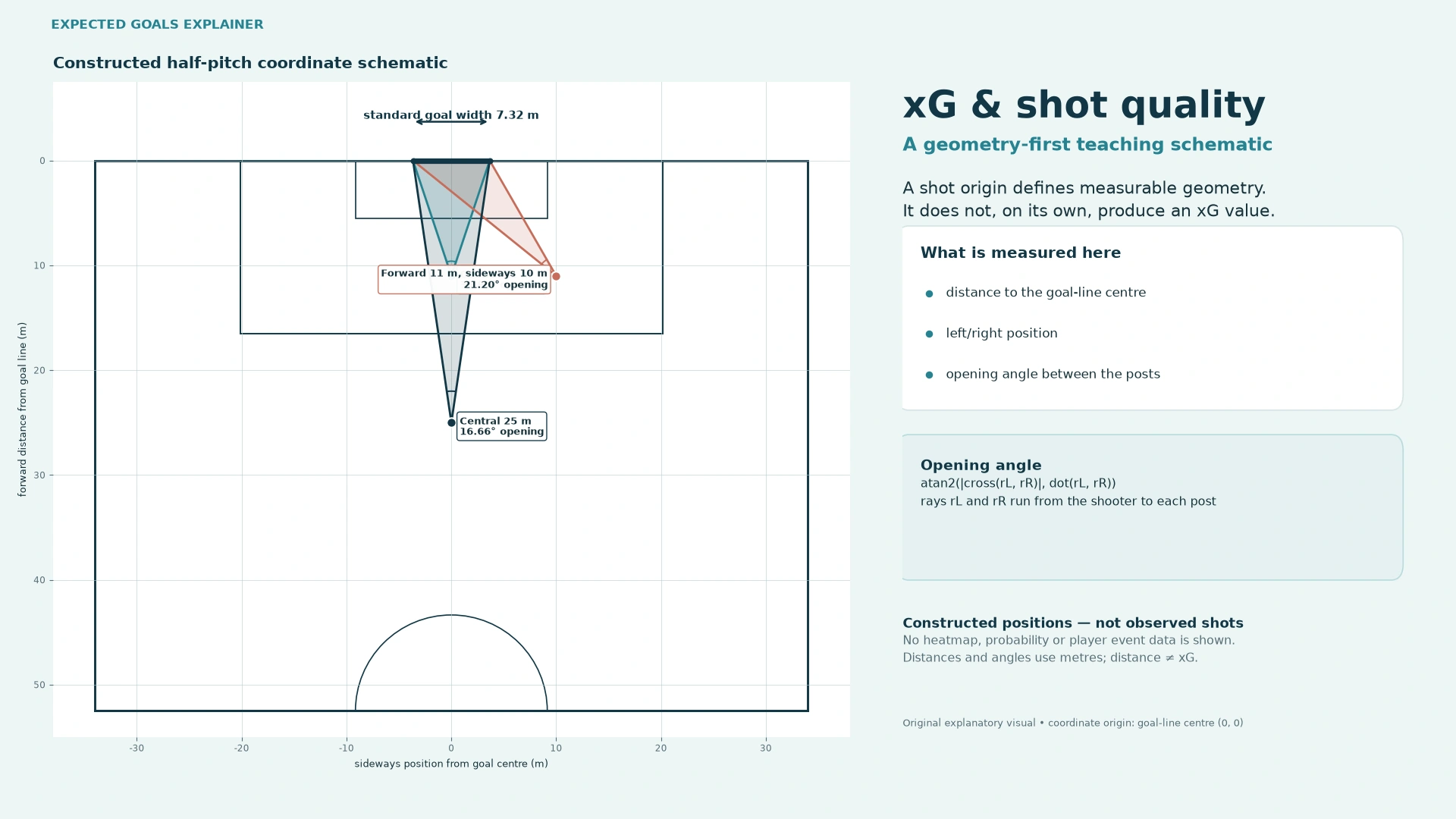
Expected Goals (xG) Explained With Real Examples

Expected goals, usually written as xG, is a model's estimate of the probability that a particular football shot will become a goal. A chance valued at 0.20 xG has an estimated scoring probability of 20%, given the information used by that model. It is not a promise that this attempt will score, and it does not tell the referee what the result should have been.

If you have watched a team win despite a lower xG total, the number can seem confusing. The explanation is simpler than it looks: a probability describes a chance before the outcome, while the scoreboard records what actually happened. This guide connects those two ideas through original shot diagrams, transparent calculations and documented football examples. You don't need a statistics background to follow it.

Start here if you want expected goals explained without treating one decimal as the whole match. For the wider context, our sports analytics guide explains how a metric becomes useful only when its meaning and limitations match the question you are asking.

Key takeaways before you read a shot map

• A shot's xG is an estimated probability, not a goal already earned.
• Team xG normally adds the probabilities assigned to its recorded shots; the total can exceed one.
• Location matters, but body part, delivery, defenders and goalkeeper context can change the estimate.
• Different data providers and model versions can produce different values for the same attempt.
• Read the shot sequence and footage alongside the total. Neither a high xG nor a low xG decides who deserved a result.

What is xG in football?

A shot has two possible recorded scoring outcomes: it becomes a goal or it doesn't. An xG model assigns a probability to the first outcome using historical shot data and contextual information. Opta Analyst's 8 August 2023 explainer describes this as estimating chance quality from similar past shots. Hudl Statsbomb's explanation uses the same central idea: compare the circumstances of an attempt with patterns learned from earlier attempts.

The word expected comes from expected value in mathematics. It does not mean an analyst is demanding a particular result. If many suitable chances were each assessed at 0.20, a well-calibrated model would expect roughly one fifth to become goals across a large sample. A single attempt still produces zero or one goal. Ten such attempts need not produce exactly two.

You can translate a decimal into a percentage by multiplying by 100. That helps explain the number, but it does not remove uncertainty about the model itself. A displayed 0.20 may be rounded, and a model may lack important context. Read it as an estimate based on defined information, not as a measurement with unquestionable precision.

The abbreviation does not describe one universal formula. It names a family of models with a shared purpose. Before comparing values from two websites, find out whether they use the same provider, time period, competition coverage and definition of shots. Two identical labels can conceal different methods.

Why shot count alone misses chance quality

Imagine two attacks. One ends with a player stretching to head a high cross from a narrow angle. The other ends with a controlled foot shot from a central position after a low pass. Both count as one attempt, but that does not make them equally likely to score. xG attempts to describe the difference that a simple shot count leaves out.

This is useful when the total number of attempts creates a misleading impression. A side can take many difficult shots while another creates fewer, better opportunities. The xG total combines quantity with estimated quality. Average xG per shot then helps separate those two ingredients: did the team create more attempts, more valuable attempts, or both?

However, the metric sees the shots that were recorded, not every promising attack. A dangerous pass that nobody reaches may produce no shot-based xG. A player losing control before shooting can end an excellent opportunity without adding to the total. The absence of xG therefore does not prove the absence of attacking threat.

A helpful report keeps these different observations together. Shot count describes volume; xG describes estimated scoring opportunities within that volume; footage shows how the opportunities arose. Our football video-analysis software comparison explains tools that can help coaches organise those clips without assuming that an automated label is already correct.

Which factors affect a shot's expected goals?

Distance and goalmouth angle are familiar starting points. Other things equal, a closer central shot generally gives a player a more favourable view of goal than a distant or sharply angled attempt. Those are tendencies learned from data, not instructions that every close shot will be easy. A defender, a bouncing ball or a rushed touch can make a nearby attempt difficult.

Body part and shot technique matter too. A header is not equivalent to a controlled foot shot from the same location. The preceding action can change what the player has time to do: a low square pass, a high cross, a through ball and a rebound present different situations. Models may encode these as shot types or assist categories, with definitions that vary between providers.

Defensive pressure, goalkeeper position and the positions of surrounding players add context. A shot location alone cannot tell whether the goalkeeper is stranded or whether several defenders obscure the goal. Hudl Statsbomb's explainer describes using freeze-frame positions and shot-impact height. Opta's dated 2023 explanation also describes goalkeeper and player-position information among its inputs. It would be inaccurate to assume that every contemporary model uses location alone.

Some relevant circumstances remain hard to observe or represent. A model may not fully capture balance, visibility, the quality of the first touch or an unusual deflection. More recorded features do not automatically guarantee better estimates. The real question is whether the data are consistent and the model performs well on appropriate unseen examples.

Original shot diagram: distance is not the whole angle

On a small screen, scroll sideways to read the diagram.

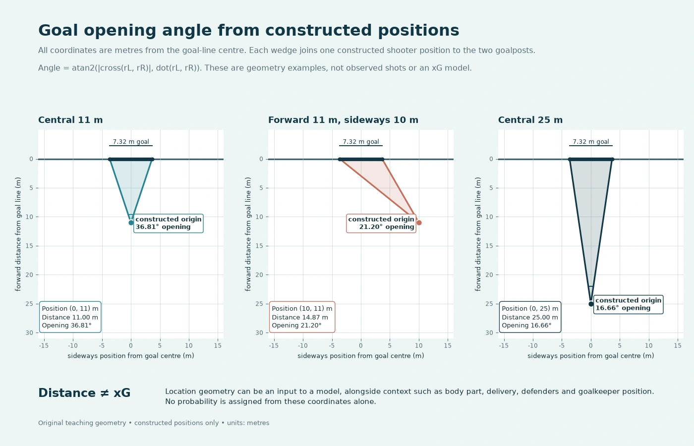
The diagram separates two quantities that viewers sometimes combine. Distance to the centre of goal is a length. Goalmouth angle is the opening between the two rays from the ball to the goalposts. Moving sideways can narrow that opening even when a shooter remains relatively near the goal line. A model can use both pieces of information rather than treating every point at similar distance as equivalent.

These constructed positions are deliberately not presented as real shots by the players discussed later. We have the published player totals, but not the shot coordinates behind them. Inventing coordinates and attaching a famous player's name would turn a useful explanation into false evidence. Here, the diagram teaches geometry and nothing more.

Nor does the diagram supply a scoring probability from the coordinates. To do that responsibly, you would need a defined, validated model and other supported inputs. Two players shooting from one point might face different goalkeeper positions, body-part requirements or pressure. A coloured location chart should not hide those differences.

When reading a real shot map, check its orientation and legend. Does each marker indicate a location, a probability, an outcome or all three? Are larger circles genuinely scaled to xG, or are they decorative? If coordinates come from video, calibration affects their interpretation; our computer vision in sports guide explains why mapping pixels onto a pitch requires care.

How expected goals are calculated by a model

The basic training problem starts with historical attempts. Each row contains features describing the shot and a label saying whether it became a goal. The model learns relationships between those features and outcomes. It then estimates a probability for a new shot from its recorded characteristics. It does not need to know the new shot's final outcome to estimate pre-shot chance quality.

An understandable first model might use logistic regression. More complex systems can use tree-based machine learning or other methods. Opta's August 2023 explainer described its then-documented model as using XGBoost with more than 20 variables. That is a dated description, not an independently verified statement that every Opta product has unchanged architecture in 2026. XGBoost's name does not make it the definition of xG.

Training is not simply counting how many goals came from an exact pixel on the pitch. Exact situations rarely repeat. A fitted model combines information across examples and interactions. For instance, the effect of a header may depend on distance and delivery rather than acting as one fixed deduction for every attempt.

After training, the model needs evaluation on data it did not use to learn those relationships. Otherwise it may reproduce historical patterns without generalising. Data quality, appropriate testing and the population represented by the training set matter as much as the sophistication of the algorithm. A larger feature list alone is not a validation report.

A transparent calculation is not a production xG formula

A logistic model converts a score into a probability using p = 1 / (1 + exp(-z)). The score z is built from fitted coefficients and features. If z were zero, the probability would be 0.50. If z were minus two, it would be approximately 0.119. These are mathematical examples, not estimates for a particular football shot.

The important part is how z was obtained. A real model needs coefficients learned from suitable labelled data, properly defined variables and validation. There is no honest way to recreate a provider's complete model by choosing a convenient distance multiplier and calling the result official xG. Even when the arithmetic is correct, the probability can be unsupported.

A useful educational calculator can instead work with probabilities that have already been assigned. That is what the calculator in this guide does. It adds values, finds their average and demonstrates a separate probability calculation under stated assumptions. It does not turn a location, a player's name or a match score into a new predicted shot value.

If you are learning analytics, keep those stages separate: data collection, probability estimation and aggregation. A spreadsheet sum is not evidence that the probability estimates were good. Conversely, a carefully fitted model can still be misused when its outputs are compared with incompatible totals. Explaining where a number came from is part of explaining the number.

Add the shots to calculate team xG

Suppose three separate recorded attempts have assigned values of 0.05, 0.15 and 0.40. Their total is 0.60 xG. This is a constructed arithmetic example, not a real team's match report. The calculation is straightforward: add the values without turning each missed shot into zero after you know the result.

A team total can be greater than one because it summarises multiple probabilities. A side recording 2.10 xG is not claiming that any individual attempt had a probability of 210%. It is describing the sum of the values of its shots. Actual goals can finish above, below or near that sum in a particular match.

For a fixed collection of shot outcomes, expectations add without requiring the outcomes to be independent. That is a different calculation from finding the probability of at least one goal. The distinction becomes especially important when discussing rebounds and alternative events within a possession, where observed attempts are conditional on how the preceding play unfolded.

Always inspect which attempts are included. Penalties, extra time, shootouts, disallowed events and later data corrections need clear treatment. A match total shown by one service should not be compared with a regulation-time-only number from another without noticing the difference. Keep the provider's definition attached to the sum.

Average xG per shot explains a different question

Average xG per shot is total xG divided by the number of included attempts. In the constructed three-shot example, 0.60 divided by three is 0.20 xG per shot. This summarises the mean estimated chance quality. It does not say that every attempt was a 0.20 chance: the individual values were very different.

The average can help when two players have different shot volumes. A player taking many attempts from difficult positions may accumulate substantial total xG while recording a low average. Another can have a high average from a small number of favourable opportunities. Neither quantity is enough to judge the player on its own.

Averages also conceal distribution. A penalty plus several long shots can have the same mean as a set of more consistent open-play chances. A histogram, shot map or clip list can reveal that difference. The average should prompt a closer look, not end the explanation.

Check the denominator carefully. If a display excludes some blocked shots from a separate shooting-accuracy statistic, that rule does not automatically apply to the xG-per-shot figure you are calculating. Stats Perform's event definitions illustrate why similarly named shot metrics can have different inclusion rules. Use the attempt count that matches the xG dataset.

Real example: Sánchez and Neves took the same number of shots

On a small screen, scroll sideways to read the diagram.

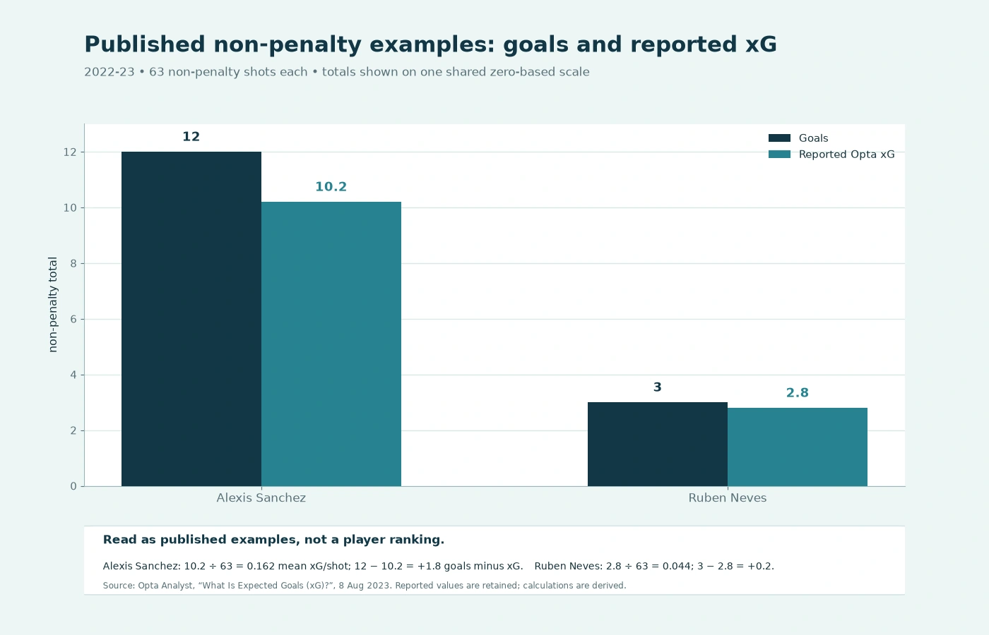
Opta Analyst provides a practical example of why shot count alone is insufficient. In its August 2023 explanation, it reports that Alexis Sánchez at Marseille in Ligue 1 and Rúben Neves at Wolverhampton Wanderers in the Premier League each took 63 non-penalty shots in 2022–23. Sánchez scored 12 non-penalty goals from 10.2 xG. Neves scored three from 2.8 xG.

Their opportunity totals were therefore very different despite equal shot volume. The source explains that Sánchez's shots came from much closer to goal. The reported xG supports the narrow conclusion that their collected attempts had different estimated scoring quality under that provider's model. It does not establish that one player was better at every aspect of football.

Our derived average is 10.2 / 63 = approximately 0.162 xG per shot for Sánchez and 2.8 / 63 = approximately 0.044 for Neves. These calculations use the rounded published totals, so they should not be presented with excessive precision. The original unrounded event values could produce slightly different last digits.

The comparison spans different leagues, team environments and player roles. It illustrates chance quality, not an experiment controlling all those conditions. Both the source year and non-penalty definition stay visible so that a reader does not mistake this for a current-season table. The downloadable summary dataset preserves those labels rather than inventing the missing shot records.

What goals minus xG can tell you about finishing

Using the same published example, Sánchez's goals minus xG is 12 - 10.2 = +1.8. Neves' difference is 3 - 2.8 = +0.2. Both scored somewhat above the quoted estimates. This does not mean the model declares their additional goals invalid. It is a comparison between observed results and estimated opportunities.

The difference can be a starting point for investigating execution. You might examine whether shots were well placed, whether the sample includes unusual events, and whether the model represents the situations well. You cannot isolate finishing skill from one subtraction. Chance definitions, goalkeepers, pressure and ordinary variation all affect interpretation.

One season is also not an automatic forecast. Repeated patterns across suitable larger samples may support a stronger assessment, but they still need contextual analysis. A player's role can change, and a new season need not contain the same opportunities. Comparing absolute differences between players with very different minutes or shot counts can further mislead.

Avoid the idea that a player who has scored above xG is obliged to miss later to repay the difference. Previous goals already happened. The relevant future question concerns the player's new chances, execution and model context. Historical overperformance is not a debt the next shot must settle.

Real example: Sterling's shot quality versus shot placement

Opta Analyst's 23 June 2021 xGOT explainer discusses Raheem Sterling's free kick against Crystal Palace at the start of 2021. It reports the opportunity as 0.10 xG, then reports 0.81 xGOT after accounting for the shot's placement towards the top-right corner. The article describes it as a goal. These numbers refer to different questions and stages of measurement.

Pre-shot xG asks how likely the opportunity was to produce a goal based on information at the attempt. xGOT, in that documented Opta definition, adds where an on-target shot was heading within the goalmouth. A low-probability opportunity can be executed in a way that is difficult to save. That does not require rewriting its original pre-shot value as 1.00 because it scored.

The increase from 0.10 to 0.81 should not be called a universal measure of pure finishing skill. Post-shot models have their own inputs and limits. Defender interventions and the set of shots included can affect aggregate interpretations. Hudl Statsbomb's model-update discussion likewise distinguishes chance quality from shot execution and goalkeeper-related questions rather than treating them as one interchangeable number.

For a viewer, the useful lesson is simple: check whether the graphic says xG or a post-shot metric. The same shot can have different justified values because the model has different information. Our original diagrams do not reconstruct Sterling's exact coordinates or flight; those details are not supplied by the aggregate example we are using.

Penalties have high xG, but not one universal constant

A penalty provides a more standardised shot setting than most open-play attempts. Providers often use a fixed value reflecting historical conversion in their relevant data. However, fixed does not mean universal or permanent. Hudl Statsbomb's explainer references a 2022 update at 0.78 xG, while Opta's August 2023 explainer quotes 0.79. Those are dated provider examples, not a recommended constant for every model.

This helps explain why match xG totals can differ. A model's handling of penalties is only one source of disagreement, but it is easy to spot. More subtle differences can arise from pressure labels, body-part definitions, keeper positioning or feature processing. Round-off in the displayed individual shots can also make their visible sum differ slightly from a reported unrounded total.

Non-penalty xG removes the penalty attempts from the stated xG total. It can be useful when investigating how a team creates chances in other phases. Keep the corresponding goal and shot counts on the same basis. Comparing non-penalty xG with goals that include penalties would mix definitions and distort the goals-minus-xG calculation.

Shootouts need separate treatment because they are not ordinary match attempts in most event summaries. Check the provider and competition display rather than assuming the scoreboard and xG panel include the same events. State exclusions explicitly, especially when extra time or a knockout decision is involved.

Try the illustrative xG arithmetic calculator

Enter probabilities that have already been assigned to separate shots, such as 0.05, 0.15, 0.40. The default example totals 0.60 and averages 0.20 per shot. You can replace the values to see how the arithmetic changes. Inputs must lie between zero and one; the tool rejects missing, invalid or out-of-range values instead of silently turning them into believable statistics.

This is an arithmetic calculator, not a fitted xG model. It does not assess a real shot from its distance or angle. It has no knowledge of a player's technique, a goalkeeper's position or a competition's data. You are supplying the probabilities; the tool only explains how to combine them.

The separately labelled at-least-one output assumes independent opportunities and uses one minus the product of their failure probabilities. It is a mathematical demonstration, not an interpretation that should be applied automatically to all observed shots in a football possession. The tool performs everything in the page without sending inputs to an external service or saving them.

To follow the guide without using the calculator, the written examples provide the same arithmetic. A useful page should not require an interactive widget to explain its core claim. The default values and limitations remain visible in the initial page, and the dataset offers a separate way to practise with sourced historical summaries.

Equal total xG can describe different collections of chances

On a small screen, scroll sideways to read the diagram.

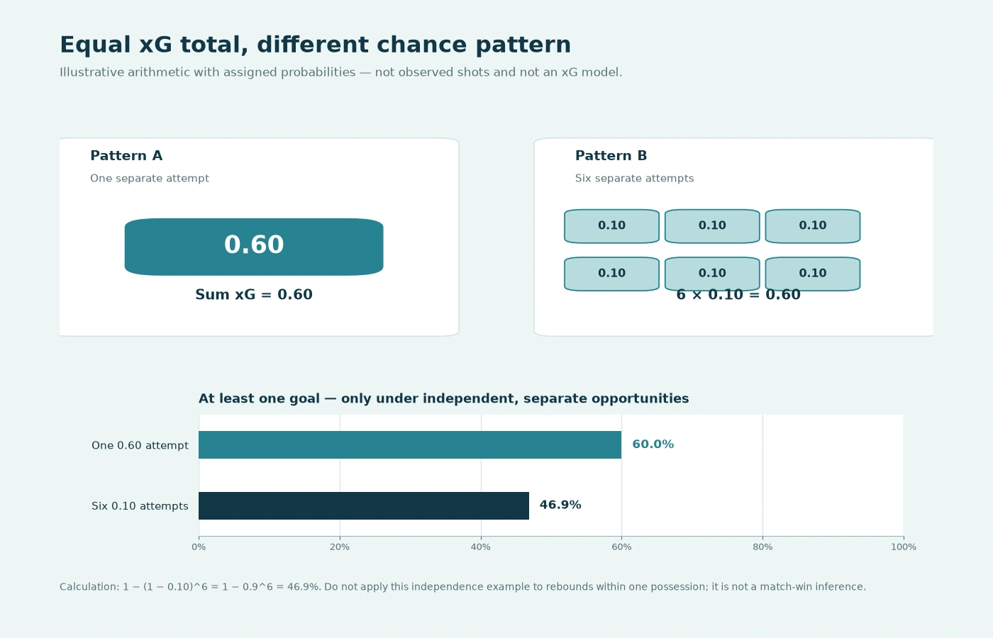
One opportunity valued at 0.60 and six separate opportunities valued at 0.10 each have the same summed xG. But their distributions differ. The first collection can produce at most one goal from its single attempt. The second collection could produce several, depending on the outcomes of its separate attempts.

Under the explicit independence assumption, the chance of none of the six attempts scoring is 0.90 multiplied by itself six times. The probability of at least one is one minus that product, approximately 46.9%. For the one 0.60 attempt, the equivalent probability is 60%. The sum of probabilities is not generally the probability of at least one success.

That difference is not evidence that one real team would necessarily win. We have not described an opponent, match state, how opportunities arise or their actual dependence. The demonstration exists to explain why a single total cannot answer every probability question. It uses constructed values rather than pretending to forecast football.

When reading a real match report, this should make you curious about the shot collection. Were the chances concentrated in one sequence, spread across the match or shaped by chasing a deficit? The total provides an entry point. The shape of the opportunities and their context explain more.

Rebounds need sequence context, not automatic independence

A rebound attempt may exist only because an earlier shot did not score and the ball remained available. Its occurrence is tied to the earlier event. Taking the probabilities of two observed attempts and treating them as independently available before the whole sequence can therefore produce a misleading estimate of the sequence's scoring chance.

For a constructed example, suppose an initial attempt has a 0.40 scoring probability. If it fails, imagine that a follow-up certainly becomes available and has a conditional scoring probability of 0.50. Under those explicit assumptions, the sequence's probability of a goal is 0.40 + 0.60 × 0.50 = 0.70. It is not 0.90 just because the two listed values add to that number. Real follow-ups are not guaranteed, so a real sequence requires additional information.

A conventional match xG total can still list and add the shot values that actually occurred. That descriptive shot total is not the same question as assessing the entire possession before it unfolds. Some providers offer sequence-adjusted measures; check the definition rather than relabelling one calculation as another.

This is why video matters. An analyst should preserve event order and identify whether a second shot came from the same attack. Our AI video-analysis guide explains event detection and human verification: a correctly summed table is not enough if the clips or event identities behind it are wrong.

Does the team with higher xG deserve to win?

Higher xG indicates a larger estimated opportunity total for the included attempts under the chosen model. It does not award a deserved result. Goals decide the score, and football includes effective finishing, saves, defensive actions and decisions that a shot-quality total does not fully represent. Opta's explainer explicitly warns against treating match xG as the expected outcome of the game.

Match state also affects what follows. A side protecting a lead may concede territory while choosing different attacking risks. A side chasing a goal may take more attempts. The final shot collection reflects that developing contest, not a controlled trial where both teams played identically regardless of the score.

Some attractive attacks produce no shot, while a brief penalty incident can add a large probability to the total. Neither fact makes xG useless. It makes the question more specific: what scoring opportunities were recorded, and how were they distributed? Describe that before turning it into an overall verdict on tactical superiority.

A balanced explanation can say that a losing team generated more estimated chance quality while acknowledging that it lost the actual match. It need not claim the score was wrong or the winner had no merit. The metric adds context to what happened; it does not replace what happened.

Why different xG models disagree

Models can use different data, feature definitions, training populations and statistical methods. One may record the goalkeeper accurately; another may use a proxy or lack that position entirely. An attempt can then receive different probabilities without either provider making an arithmetic mistake. The disagreement may reflect information, assumptions or model quality.

Model versions matter too. Statsbomb's May 2022 upgrade discussion explains changes to blocker and goalkeeper representation, including smoother relationships around position boundaries. Historical values available today may not be identical to values first displayed during a match. An analyst needs the relevant data version, not just a familiar provider name.

Comparing a small difference between two services can be less informative than it appears. The values may be rounded, shots may be classified differently, or one feed may have been corrected later. First align the event set. Then investigate features and documented method differences before declaring a precision contest.

For season comparisons, use a consistent provider and version where practical. If you must combine sources, clearly mark the break rather than presenting the full series as directly interchangeable. Our data contracts for performance teams explains why definitions and change records make a dataset more useful over time.

How to judge model reliability and sample size

Calibration asks whether groups of shots assigned similar probabilities score at approximately those rates across suitable samples. A model could rank easier shots above harder shots reasonably well while its probabilities are systematically too high or low. Ranking quality and probability reliability are related questions, but they are not identical.

One match cannot establish whether a model is calibrated. A shot valued at 0.05 can score without disproving the estimate. Conversely, one missed 0.80 chance is not evidence that the model is useless. Evaluation needs enough appropriate examples, careful separation of training and test data, and attention to where errors occur.

The population matters. Men's professional, women's professional and academy football can have different data distributions. Opta's August 2023 article describes a separately retrained women's-competition model rather than simply assuming that every learned relationship transfers unchanged. This is a sourced example of why model applicability should be checked, not a claim that all providers use the same approach.

For a youth team, avoid pretending that a public professional-football value is a personalised truth about each child. Use the framework to discuss opportunity quality, but be honest about absent local validation. Our football scouting across India's competition contexts discusses the wider problem of making comparisons across different environments.

Common xG misconceptions to stop repeating

“A goal must have 1.00 xG.” No. That would confuse the known outcome with the probability assessed before it. A difficult shot can score; a favourable opportunity can fail. The pre-shot estimate should not simply be replaced by the final label if it is meant to describe chance quality.

“xG only counts shots on target.” Do not assume that. Pre-shot models can value attempts that later miss or are blocked, according to the provider's shot definitions. Post-shot and on-target models answer different questions and often have a narrower event set. Reading the abbreviation and method prevents this mix-up.

“The highest total proves the best player or team.” A total summarises included opportunities. It does not directly measure passing choices, off-ball movement, defensive contribution or every aspect of finishing. Even xG per 90 minutes needs role, competition, minutes and sample context before supporting a comparison.

“More decimal places mean more certainty.” A model can output many digits while its features contain uncertainty. Use sensible display rounding, retain exact source values for calculations when available, and avoid describing an estimate as precise beyond the evidence. A readable report is usually more honest than an unexplained string of decimals.

A practical way to read xG statistics

Begin with the source and period. Identify the provider, match or season, included minutes, penalty treatment and any revisions. This takes less time than arguing about two totals that describe different event sets. In the real player example here, the correct label is Opta's published 2022–23 non-penalty comparison, not a current ranking.

Next, inspect volume and quality together. Read total shots, total xG and average xG per shot, then look at their distribution. A single headline number can hide one large opportunity or many small ones. If the question concerns finishing, add actual goals and suitable execution evidence rather than assuming a subtraction explains everything.

Then review the important clips. Confirm player identity, shot location, body part, delivery, defensive pressure and event order where the data allow it. Where a video angle does not show enough, retain that uncertainty. Our video tagging workflow explains how to organise review so that a report remains connected to observable play.

Finally, write one appropriately narrow conclusion. For example: the recorded attempts had higher estimated chance quality under this model, with the difference concentrated in particular sequences. That is more useful than announcing that a decimal has proved a complete theory of the match. A good metric should help you ask a better next question.

Questions readers ask about expected goals

Can an individual shot have more than one xG?

An individual scoring probability lies between zero and one. A team or player total can exceed one because it adds values from multiple shots. Check whether a displayed figure refers to one attempt, a sequence or a match before interpreting it.

Can a team have xG without scoring?

Yes. Probabilities do not guarantee outcomes, so a collection of opportunities can finish with no goals. Use the clips and model context to investigate why; do not assume a particular explanation such as poor finishing solely from the total.

Is xG the same as expected assists?

No. Expected assists evaluates a different action and needs its own provider definition. A pass-based metric is not simply interchangeable with a shot-based probability. Read the action, training target and aggregation method before comparing them.

Can this calculator assess my own football shots?

It can add probabilities you supply, but it cannot validate those probabilities or calculate a shot's quality from a photograph. It is a teaching tool for arithmetic. Real assessment needs a defined model, suitable input data and review of its applicability.

Which xG model should I use?

Use a documented model that fits the dataset and question, and keep the source consistent where possible. Evaluate definitions, coverage, validation and versioning rather than selecting whichever single-match total agrees with your preferred interpretation.

What to take from the number into your next match

Expected goals makes a familiar observation more structured: not all shots are equally favourable. Its value comes from combining that observation with a clear probability estimate, a known method and a record of the opportunities behind it. You can appreciate a remarkable finish while recognising that the original chance was difficult.

The two real examples show why labels matter. Sánchez and Neves illustrate different opportunity quality within equal shot counts. Sterling illustrates the separation between an opportunity and its on-target execution. Neither example licenses a universal player ranking or a promise about what comes next.

Keep the calculator, diagrams and dataset in their proper roles. The diagrams explain geometry; the calculator explains arithmetic; the historical summary gives a retrievable example. The sports analytics guide is the next step if you want to connect these numbers with a broader coaching question. Let evidence improve the conversation rather than make it less thoughtful.

Page metadata and source notes

SEO title: Expected Goals (xG) Explained: Meaning, Calculation and Examples. Meta description: Understand expected goals with real football examples, shot-quality diagrams, clear xG calculations, model limitations and an illustrative arithmetic calculator.

Primary keyword: expected goals explained. Related terms: what is xG in football; how expected goals are calculated; xG statistics explained. These identify the page's educational intent, not measured monthly volume or a ranking guarantee.

Sources reviewed on 13 October 2026: Jonny Whitmore's Opta Analyst xG explainer, dated 8 August 2023; his xGOT explainer, dated 23 June 2021; Hudl Statsbomb's undated xG explanation; Dinesh Vatvani's Statsbomb model-update article, dated 15 May 2022; Stats Perform's Opta Event Definitions; and IFAB Law 1 for goal dimensions. The historical player aggregates and Sterling example are attributed where discussed. External provenance URLs remain in the private research record; visitor links stay on SportyTechs.

The shot positions, three-shot arithmetic, equal-total illustration, logistic example and rebound calculation are constructed teaching examples, not observed SportyTechs match or athlete data. No trained model, provider-comparison test or personal performance prediction was produced. The calculator combines entered probabilities only. Historical model descriptions are dated rather than presented as independently verified 2026 product specifications.